
The Molecular World Through A New Lens: How Cryo-EM Works
- StemSide

- Apr 23, 2021
- 23 min read
Updated: Jun 20, 2023
Authors’ note: we also recommend checking out this article in Primer on X-ray crystallography for some background information on structural biology.
Several years ago, a revolution was quietly sweeping through the field of structural biology. A technique called cryogenic electron microscopy (cryo-EM) was beginning to rise to prominence. More and more articles were being published, showcasing protein structures that had been solved with this technique. In addition, many of these protein structures had been challenging to solve with X-ray crystallography and nuclear magnetic resonance (NMR) spectroscopy – the primary methods of protein structural determination at the time.
Nowadays, cryo-EM is one of the jewels in the crown of structural biology and is set to improve even further. To understand why this is the case, we must explore this technique in detail.
What is cryo-electron microscopy?
Generally, electron microscopy encompasses a variety of techniques where electrons are used as the source of illumination to image materials. In biology, two methods of electron microscopy are commonly used:
Scanning electron microscopy, where an electron beam passes across the surface of the sample only.
Transmission electron microscopy, in which electrons pass through the sample to form an image in a way similar to light microscopy.
On that note, cryogenic electron microscopy (cryo-EM) is a form of transmission microscopy. However, what distinguishes it from other electron microscopy techniques is that samples of proteins or cells are rapidly plunge-frozen to encase them in vitreous (meaning ‘non-crystalline’) ice. Once the proteins are frozen, they can be imaged with an electron microscope. Typically, many images of the sample protein are taken, which can then be used to reconstruct its 3D structure.
We’ll go into more details of this process later in the article. But first and foremost, we will look at what made this technique so revolutionary.
Why bother with this technique?
It may not be apparent why cryo-EM has caused such a stir in structural biology. Indeed, for many years, the quality of protein structures from electron microscopy was much worse than those from X-ray crystallography, thereby suggesting that its applications were quite limited.
A key improvement was the implementation of the plunge freezing technique as mentioned earlier. However, even with this improvement in sample preparation, it took many years of gradual development before structures comparable to crystallography and NMR could be obtained. In fact, the recent ‘resolution revolution’ was an accumulation of many improvements to sample preparation, electron microscopy hardware, and image processing software.
Of course, this begs the question of ‘why was there so much work put into improving cryo-EM?’.
Experimentally speaking, the main reason is that X-ray crystallography and NMR are limited at solving protein structures, a task fundamental to understanding biological function. More specifically, NMR is limited in studying proteins larger than ~26 kDa while X-ray crystallography requires proteins to be crystallised – a much harder task than it may seem. And that’s because many proteins of interest form large complexes which are difficult to crystallise, with common examples of these including ribosomes, membrane proteins, and cytoskeletal proteins.
The importance of this is that proteins rarely function on their own since many functions depend on proteins forming complexes with other proteins. So, being able to characterise the structures of these complexes is essential to characterising their function. As a result, the ability of cryo-EM to determine the structures and functions of these large protein assemblies is a major advantage over other experimental techniques.
Beyond experimental techniques, computational prediction of protein structure has made huge strides in recent years too. Notably, Alphafold performed exceptionally well in the past two assessments of structure prediction, with some headlines even claiming protein folding was solved. Therefore, one may wonder whether experimental structural biology is even necessary anymore. However, one of the structures that Alphafold struggled to predict existed as a protein complex – the types of structures amenable to analysis by cryo-EM.
There is also a variant of cryo-EM called cryo-electron tomography (cryo-ET) that looks to examine protein structures in situ, i.e. in their native cellular environment. Even with the power of Alphafold, structural prediction methods are not yet able to do this. While the structures from cryo-ET are not yet of the same quality as ‘traditional’ cryo-EM, research is ongoing to improve this. Hence, cryo-EM is likely to remain a major player in the field of structural biology in the years to come.
How does it work?
Now that the benefits and advantages of cryo-EM have been laid out. We are now ready to take an in-depth look at what makes this all possible.
As hinted earlier, every step from sample preparation to image processing, as well as all the components, play a role in obtaining the high-quality structures that are now ubiquitous in scientific journals.
However, to understand why each step, or component, helps in determining protein structure, we must first look at some of the physical principles behind cryo-EM.
Physical principles
Properties of electrons
To start with, it is important to note that electrons exhibit wave-particle duality. The actual interpretation of this is quite complicated and will not be discussed, but essentially what it means is that electrons can be described as waves as well as particles.
As a result, they have properties such as amplitude, wavelength, frequency, and phase shift. These are illustrated below:
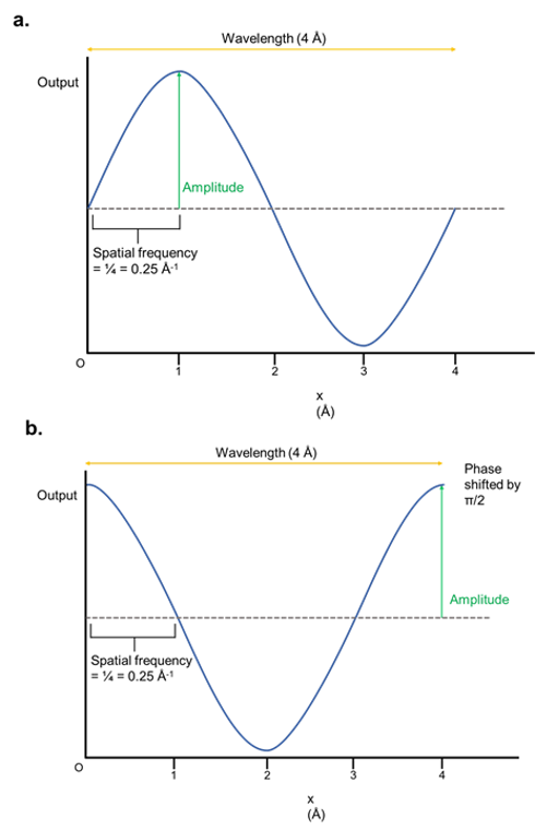
Figure 1: The properties of waves. (a) A sine wave that varies with x, which signifies the distance from an origin point. The y-axis is depicted with an arbitrary output. In practice, this output is usually the intensity/brightness of the wave. The wavelength is the length of one complete cycle. The amplitude is the maximum output of the wave function, and the spatial frequency is the fraction of a wave completed per unit of distance (shown in angstroms). (b) The wave is identical to (a) except that it has been phase-shifted by π/2, which basically means it has been horizontally shifted.
It is also important to note that when structural biologists refer to ‘waves’, particularly electron waves, they are slightly different from the waves that are often encountered in introductory physics classes.
Typically, waves are first introduced as some kind of output that oscillates with time. For example, sound can be described as oscillations of air pressure that vary with time.
On the other hand, instead of varying temporally (i.e. varying as a function of time), the waves in structural biology often vary in space only. In other words, the output oscillates across a distance instead. What this means is that the frequency of electrons in cryo-EM is not described in units of hertz, which would denote the number of cycles per second. But rather, it is a spatial frequency that is the inverse of the wavelength and hence, described in units of inverse length, e.g. nm^-1.
Essentially, it tells us the number of waves completed per unit of length. For example, a wave with a spatial frequency of 2 nm^-1 means that two waves are completed per nanometre. As we will see later, describing electrons as waves is a convenient way of explaining image formation, as well as explaining how certain parts of an electron microscope work.
Why electrons?
It has been known for many years that electrons have the power to resolve structures of biological molecules because they interact strongly with the atoms. This interaction is known as scattering and can be elastic or inelastic.
Simply put, elastically scattered electrons retain their kinetic energy after interacting with the sample. In contrast, inelastically scattered electrons deposit energy on the sample, damaging it and resulting in a decrease in the kinetic energy of the electron. Elastically scattered electrons contribute to the signal which is defined as useful information that allows the 3D structure to be obtained. In contrast, inelastically scattered electrons contribute to noise - unhelpful information which does not encode information about the structure. The reasons for this will become clearer in later sections.
After the electrons have been scattered by the sample, they are refocused by the lens to form images that are 2D projections of the sample. More precisely, the scattered electrons represent the Fourier Transform of the protein molecule and refocusing by the lens performs the inverse Fourier Transform, producing an image (Figure 2). Further information on this is proved by this link but in simple terms, the scattered electrons encode the structural information of a protein.
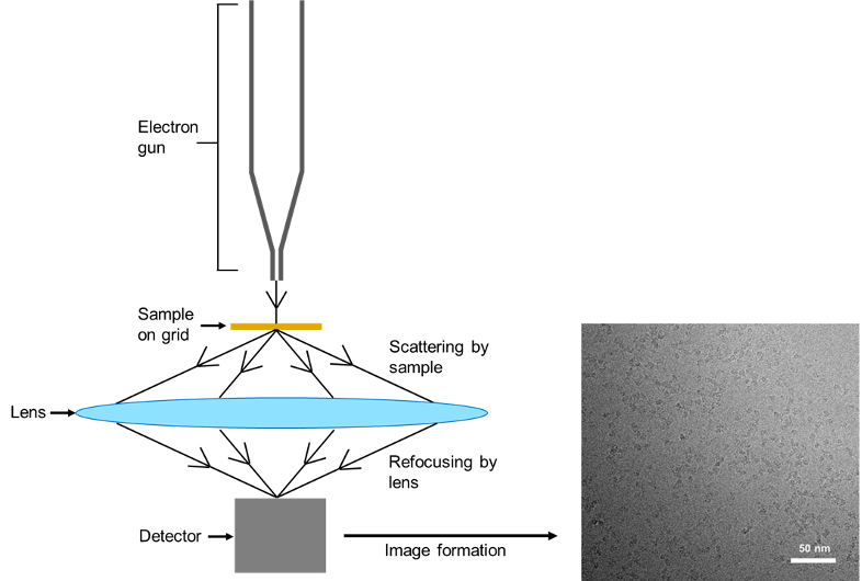
Figure 2: Scattering of electrons by proteins. Electrons emitted from an electron gun are scattered by the protein on the grid. The electrons are refocused and detected, resulting in the formation of images of the protein. The images of proteins can then be used to determine the structure. Here, an image of the SARS-CoV-2 RNA polymerase bound to an inhibitor from an article published by Yin and his team is used as an example.
Because electron scattering is what allows us to gain 3D information, this brings us to another benefit of using electrons. At the typical acceleration voltages for electron microscopes (~200 kV), the wavelength of the electrons is very short – around 2.5 picometres or 0.025 angstroms (NB: 1 angstrom = 0.1 nm and the symbol is Å).
Why this matters is because the wavelength used affects the resolution of the final structure.
What is resolution?
Resolution is a central concept in structural biology and refers to the smallest length scale that can be observed in the final structure. It is a key factor in determining what structural information can be obtained from a model, as higher resolutions mean that finer details can be distinguished.
What is slightly confusing about this is that smaller length scales correspond to a higher resolution. As an example, a 1.5 Å resolution structure has a higher resolution than a 2.5 Å resolution structure. This is because more details can be distinguished if smaller length scales can be observed. To illustrate, the length of a carbon-carbon covalent bond is roughly 1.5 Å. So, a 1.5 Å resolution structure would be able to distinguish each carbon atom while a 2.5 Å resolution structure would not.
As a rough guide, ‘atomic resolution’ refers to ≤ 1.2 Å which corresponds to the resolution where individual atoms can be resolved. Low resolution usually refers to structures > 4 Å. The definitions of ‘near-atomic resolution’ and ‘high resolution’ are less clear and both terms are used quite loosely. Rather than debate semantics, we will instead illustrate some examples of features that can be resolved at different resolutions (Figure 3).
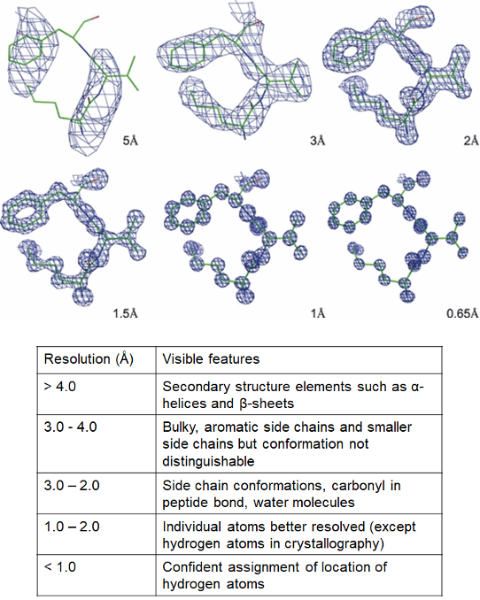
Figure 3: Different features observable at different resolutions. Electron density - the space where electrons are likely to be present - is depicted as a blue mesh and the protein chain is depicted in stick form, with carbons in green, oxygens in red and nitrogens in blue. Individual atoms are clearer at higher resolution. Images of electron density borrowed from a review by Wlodawer and his team.
As an aside, the above figure actually shows the different resolutions of structures resolved by X-ray crystallography (and not cryo-EM). Technically speaking, resolution in cryo-EM structures is calculated differently, but it can be used to correlate with X-ray structures. Meanwhile, it is important to remember that electrons from the microscope can be scattered by nuclei and the electrons surrounding the atoms, as opposed to how photons in X-ray crystallography are scattered by electrons only. Therefore, the mesh in Figure 3 would represent the locations of both the negatively-charged electrons and positively-charged nuclei for cryo-EM structures (instead of electron density only).
The reason why the short wavelength of electrons matters is because shorter wavelengths are required to resolve smaller features. This is why light microscopy, where the wavelength ranges from around 400 nm to 700 nm, cannot resolve atomic structures of proteins where distances between atoms typically range from 100 pm to 150 pm (1 Å to 1.5 Å). However, the wavelength is only a theoretical limit and even modern cryo-EM comes nowhere close to sub-angstrom resolution.
In practice, resolution is often limited by experimental factors such as inherent imperfections in microscope lenses and electrons damaging the sample. More details will be mentioned later but one important consideration is that electrons are scattered by protein molecules in solution as opposed to proteins in a crystal. Crystals have many identical proteins packed closely together, so scattered electrons (or X-rays in X-ray crystallography) are amplified, and the signal is stronger. In solution, there are usually fewer protein molecules and they are more spread out.
Therefore, one must obtain many images of proteins to get high-resolution structures, but this runs the risk of damaging the sample, increasing the noise (unhelpful information), and worsening the resolution. Thus, there is a trade-off between trying to increase the signal and increasing the noise.
For many years, low signal-to-noise ratio has haunted cryo-EM and hampered the routine acquisition of protein structures with resolutions comparable to crystallography and NMR. Nowadays, cryo-EM can easily do this and has even reached atomic resolution. To understand why, we will now examine sample preparation and the different components of a modern electron microscope.
Sample preparation
Protein expression and purification
The first step towards determining the structure of a protein is to obtain a sample of the protein of interest. This is typically done by recombinant expression, where the protein is produced in specialised live cells instead of its natural source. One major advantage of recombinant expression is that the protein of interest can be produced in a controlled environment in large amounts.
More specifically, the gene coding for the protein is first cloned into a piece of circular DNA, known as a plasmid. The plasmid (or 'expression vector', as it now carries the gene to be expressed) is transferred into cells cultured specifically for producing proteins for structural and biochemical studies. These cells are known as the expression host or expression system.
The most commonly used expression system is the bacterium E. coli; but other systems such as insect cells and even human cell lines are also used, especially for more complex eukaryotic proteins. Once the expression vector is inside the host cell, the host cell transcription-translation machinery can start synthesising the protein according to its DNA template.
Once the desired yield is reached, the cells are harvested, and the proteins of interest purified from host cell lysate. This is often done by several rounds of chromatography to obtain a pure protein sample.
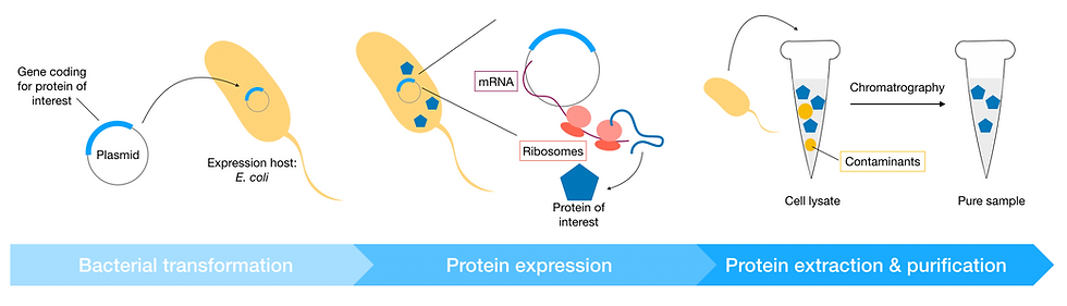
Figure 4: Schematic of recombinant expression workflow. The expression host is first transformed with the expression plasmid (a piece of circular DNA carrying the gene coding for the protein of interest). Enzymes in the host cell transcribe the plasmid DNA into mRNA; host cell ribosomes then use the mRNA as a template to synthesise the protein of interest. Finally, proteins are extracted from the cell. The cell lysate at this point still contains contaminants (often proteins from the host cell) and needs to be purified by chromatography.
One caveat to recombinant expression is that not all proteins can be easily produced in one of the commercially available expression systems. This could be because the protein is an enzyme that produces compounds toxic to the host cell, or that it aggregates when produced in large amounts. When this occurs, the protein is often purified from its natural source. Fortunately, cryo-EM can be done using a very small amount of sample protein, making it a suitable technique for proteins that are difficult to recombinantly express.
Grid preparation and vitrification
Sample preparation is crucial for obtaining high-quality cryo-EM data. Therefore, the purified protein sample needs to go through specialised preparation steps before it is mounted onto the electron microscope.
The sample solution is sprayed onto a metal mesh grid (usually copper or gold), the excess solvent blotted away, and the grid rapidly plunged frozen in a cryogen. This rapid sequence, sometimes carried out by an automated system such as a Spotiton robot, freezes the sample protein within a thin layer of vitreous ice.
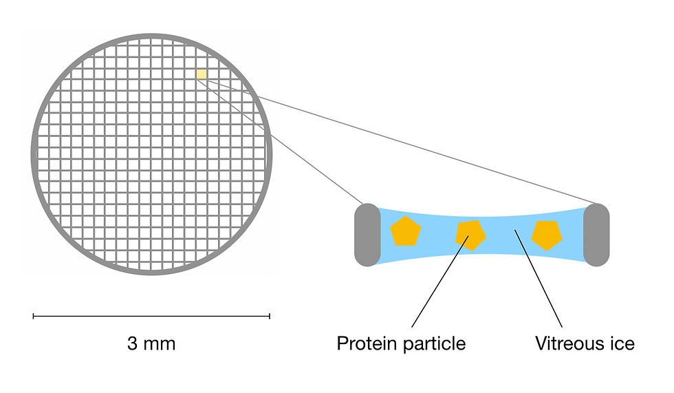
Figure 5: Schematic of a cryo-EM grid. Each hole in the mesh grid contains sample protein particles frozen in a thin layer of vitreous ice. This figure was adapted from Sgro & Costa (2018).
But first, what is vitreous ice and why is so important to cryo-EM?
Recall that water normally forms hexagonal crystals when it freezes into ice, which can damage the delicate protein specimen and generate an overwhelming amount of noise during the later data collection process. In contrast, vitrification is when the solution is rapidly cooled to liquid ethane temperatures (-188 ºC), forming glass-like (or vitreous) ice, which lacks ordered crystal structure. The vitreous ice hydrates the specimen and protects it against the electron beam without generating noisy data. In fact, Jacques Dubochet, the developer of the technique shared a third of the Nobel Prize in Chemistry 2017 since vitrification is critical to the development of cryo-EM.
To improve the resolution at the sample preparation stage, the specimen is supported by EM grids. These are tiny metal mesh grids that have a diameter of 3 mm. When the specimen adsorb onto the grids, it forms a thin layer that is only as thick as the protein itself. This is advantageous because when collecting 2D projections of 3D protein molecules, multiple molecules stacked upon one another would reduce the quality of data. To this end, additional foils such as amorphous carbon films are used to help with protein adsorption. Furthermore, different grid material and new grid designs are constantly being developed to limit specimen movement during data collection, further improving the final resolution.
Data collection on an electron microscope
Once the specimen has been prepared, it is imaged using an electron microscope. With the constant improvement of both cryo-EM hardware and data processing software, protein structures can now be solved with increasing molecular detail.
In this section, we will look at key components of an electron microscope to understand how structural data is collected, and how each component contributes to improving the resolution.
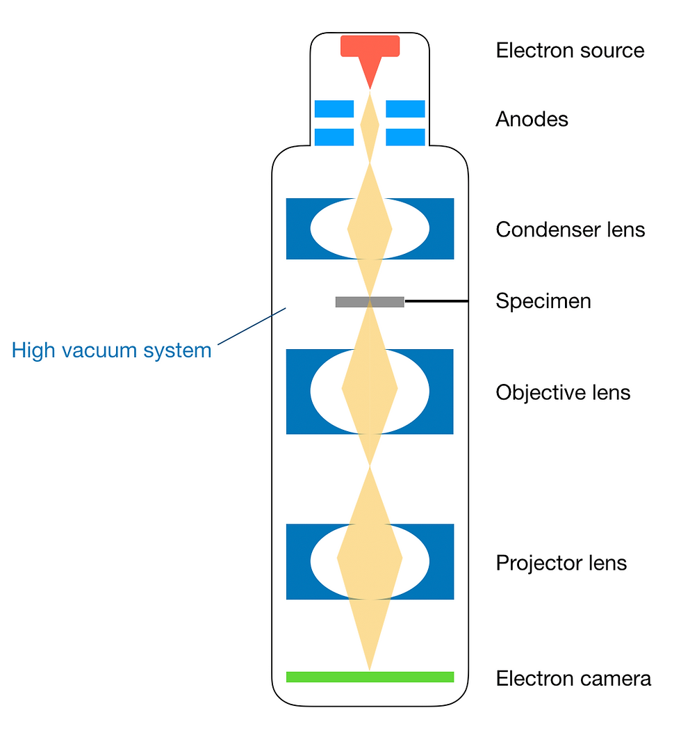
Figure 6: Schematic of major components of an electron microscope. This figure was adapted from Tanaka (2017).
Electron gun
The electron gun, as the name suggests, produces electron beams used for imaging the protein. This is no trivial task, since not only are very high voltages required, but the electrons produced also need to be spatially and temporally coherent.
Spatial coherence refers to electrons being generated at the same point, therefore travelling in the same direction. Meanwhile, temporal coherence refers to electrons having the same wavelength (recall that an electron can behave as both a particle and a wave). A coherent electron beam is curial since spatially and temporally incoherent electrons will generate a blurry image of the specimen.
Electrons are generated either by thermionic emission or field emission. In a thermionic emission gun, a tungsten filament or lanthanum hexaboride (LaB6) crystal is heated by an electric current, providing the electron with enough energy to escape the surface. In contrast, field emission guns (FEG) use a strong electric field from a sharp tungsten emission tip. Since the tungsten tip is extremely sharp (consisting of only a few atoms!), electrons produced by this method are more coherent than by thermionic emission. Therefore, modern electron microscopes are often equipped with FEGs for high-resolution cryo-EM.
Additionally, the electron gun contains an anode (positive electrode), which attracts and accelerates electrons towards the specimen. Below the electron gun, a series of condenser lenses and apertures further focuses the electron beam before it reaches the specimen.
Biological sample
The protein sample, now adsorbed onto a support grid and vitrified, is placed into the electron microscope via a specimen port. As mentioned previously, in transmission microscopy, the electron passes through the sample. It is the interaction between the electrons and atoms in the protein molecule that provides information about its structure.
As an electron passes through the specimen, it is either unscattered (i.e. does not interact with the specimen), elastically scattered or inelastically scattered. Elastically scattered electrons change direction near nuclei without losing energy, thereby providing information on the locations of atoms in the protein. Inelastically scattered electrons, however, lose energy as they interact with orbital electrons, breaking covalent bonds. In fact, inelastically scattered electrons cause radiation damage to the specimen and generate noise in the data, therefore, they are often removed by energy filters before reaching the image plane.
Additionally, only a small proportion of electrons is elastically scattered, providing useful structural information; whilst the majority of electrons is unscattered. This contributes to the low signal-to-noise ratio of cryo-EM experiments. Therefore, special techniques are required to enhance the signal during later data processing.

Figure 7: Interaction between electrons and atoms in the specimen (please note that the electrons and nuclei were not drawn to scale). (a) The electron is unscattered by the atom. (b) The electron is elastically scattered by the atom. It changes direction near the nucleus but does not lose energy. (c) The electron is inelastically scattered by the atom. It interacts with orbital electrons and loses energy. This last type of electron needs to be filtered out.
It is worth noting that electrons could also be easily scattered by air particles, creating noise. To avoid this, the entire electron microscope column is maintained under a high vacuum. The high-vacuum system also prevents air particles from being attracted to the specimen, which is kept at cryogenic temperatures throughout the experiment.
Electron lenses
Similar to light microscopy, lenses are central to the imaging process in cryo-EM. However, unlike lenses in a light microscope, electron lenses are not made of glass since they will scatter rather than focus the electrons. Instead, electrons are focused by electromagnets made of coils of wires.
As electrons travel through the magnetic field at the centre of the coil, they experience a force, sometimes known as the Lorenz force, which changes their direction of travel. This force depends on the charge and velocity of the electron as well as the magnetic field. When properly calibrated, electrons spiral towards the centre of the coil where they are focused.
We have already discussed the objective lens, which focuses the electron beam from the source onto the specimen. After being scattered by the specimen, the electrons are focused by the objective lens to produce 2D projection images of the specimen. This image is further magnified by the projector lens before it reaches the image plane.
Finally, the electron lens introduces spherical aberration where highly scattered electrons (electrons that travel close to the periphery of the lens) are over-focused. This inevitably compromises image quality, however, spherical aberration also contributes to generating contrast, specifically, phase contrast.
The contrast of images generated by an electron microscope is described by the contrast transfer function. Essentially, a contrast close to one allows high-resolution reconstruction of the specimen structure, whereas a contrast of zero means that the details are completely lost. The contrast transfer function can be manipulated by adjusting the microscope defocus. More recently, this can also be done by Volta phase plates, retrieving the data required for constructing high-resolution structures.
Electron cameras
Last but not least in the electron microscope is the electron camera. This is where structure data carried by the electrons are collected. The data collection process is digital, so the accuracy of recording where each electron hits the detector contributes greatly to final resolution.
Electron cameras initially used photographic film, which was later replaced by CCD (charge-coupled device) cameras. In CCD cameras, electrons first hit a scintillator, which converts the electrons to a light signal. This light signal travels through fibre optics to be detected by the CCD sensor. The signal detected is converted to an electric signal and stored as image data. As one might imagine, the use of light as an intermediate generates a lot of noise, as electrons are scattered by the scintillator and some light is also scattered in the fibre optics.
As a result, modern electron microscopes use direct electron detectors instead of CCD cameras. Direct electron detectors, as the name suggests, converts electrons hitting the detector (electron events) directly to an electric signal. This greatly improves the signal to noise ratio increasing the resolution.
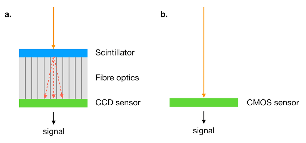
Figure 8: (a) In a CCD camera, the electron beam (orange) is converted to light (red) by the scintillator. The light is transmitted by fibre optics to the CCD sensor and converted to an electric signal. (b) In a direct electron detector, the electron beam (orange) is converted to the electric signal by the detector (CMOS sensor).
Major factors limiting the resolution at the detector are the pixel size and frame rate. The goal is to precisely locate each electron event and distinguish one electron event from the next. To achieve this, fine-tuned direct electron detectors are combined with specialised data collection algorithms such as counting mode.
The ability to collect structurally informative data was crucial to Nobel laureate Richard Henderson’s early works on cryo-EM. Nowadays, next-generation electron cameras continue to revolutionise the field, contributing to the achievement of atomic resolution structures.
Data processing
Now the final piece to the puzzle, how do we go from images collected on an electron microscope to 3D structures of proteins?
The groundwork to processing cryo-EM data is laid by Nobel laureate Joachim Frank and continues to evolve today. This section will cover the basic steps of single-particle analysis where 3D structures are constructed for a specific protein.
Firstly, distortions to the images are corrected for, using parameters such as the contrast transfer function as mentioned previously. Then, images of protein particles are picked from noise and other artefacts. A template dataset, either manually picked or taken from previous low-resolution structures, is used to select protein particles. However, it is crucial that the template is not overly detailed. This is because patterns resembling the template can be derived even from noise with no structural relevance, leading to a phenomenon known as 'Einstein from noise'.
Once the particles are picked, they are aligned and classified into different groups. Recall that the 3D protein molecule can be in any orientation in solution, resulting in different 2D projection images. Additionally, since cryo-EM has a low signal-to-noise ratio, averaging multiple images of the same class can improve this and subsequently improve the final resolution. Ideally, a large number of particles would provide high-resolution class averages. However, this is limited by the time required to collect the data and the computational power required to process this large dataset.
A 3D model of the protein can now be constructed from the 2D class averages. However, this is not the end, the 3D models still need to be classified in silico, (i.e. using computer programs) to separate different conformations of the protein. This is because merging multiple conformations can compromise the accuracy of the model.
Finally, the structure needs to be validated. A key “gold standard” method is the Fourier shell coefficient (FSC) where the full dataset collected is split into two and processed independently. This way, two structural models are built and subsequently compared in the Fourier space. In a reliable structure, the overall shape of the models should be close to identical, but the finer details would start to diverge. This is quantified by the FSC. Furthermore, a threshold FSC is set to determine the resolution (level of detail) of the structure.
Cryo-electron tomography
Up until now, what has been described is what usually comes to mind when structural biologists talk about cryo-EM. The technical term for this process is ‘single-particle analysis’. However, there are several other useful structural techniques that involve electron microscopes. One that is rapidly gaining popularity is cryo-electron tomography, or cryo-ET for short.
The main principle behind tomography is to use penetrating waves, such as electrons and X-rays, to obtain slices or cross-sections of a 3D object. These slices are taken at different angles and then combined in a process called tomographic reconstruction, resulting in a 3D image of the sample.
A common everyday application of tomography is a computed tomography scan (CT scan). Here, X-rays are applied at different angles to obtain cross-sectional images. Putting together these images allows doctors to visualise the inside of the body and thereby make diagnoses.
Similarly, in cryo-ET, the sample is plunge-frozen just like single particle analysis and placed on a grid. Collecting images is similar to single particle analysis, but a key difference is that the grid is tilted across a range of angles, resulting in images of the sample being taken at different angles (known as a tilt series).
A diagram of the experimental setup is shown in Figure 9.

Figure 9: An overview of how cryo-ET is used to study cells. Images of the cell are collected while the grid is rotated along a horizontal axis. The collected images are referred to as a tilt series. Computational reconstruction then produces a 3D structure of a cell of interest.
Rather than imaging protein molecules like single particle analysis, this method is mostly used to image the interior of cells. Prokaryotic cells, such as bacterial cells, are ideal for this because they are less thick compared to eukaryotic cells. For example, yeast cells and mammalian cells. The thickness of the cell matters because electrons are easily scattered by atoms, so thicker samples have more noise thus a poorer signal-to-noise ratio. Despite this, eukaryotic cells can still be visualised by focused ion beam milling, where a beam of ions is used to slice off the top and bottom of eukaryotic cells, leaving behind a thin layer that can be imaged with cryo-ET.
This is illustrated below:
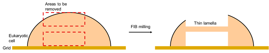
Figure 10: An illustration of FIB milling applied to a eukaryotic cell. A beam of ions is used to remove parts of a eukaryotic cell, leaving a thin lamella, which can be analysed with cryo-ET.
Overall, cryo-ET is a very powerful tool in cell biology as it can be used to examine cellular components in detail. However, its real power lies in the next technique we shall discuss: subtomogram averaging.
Subtomogram averaging
Subtomogram averaging can be considered as a subset of cryo-ET but it shares similarities with single particle analysis too. Unlike cryo-ET, the objective of this technique is to obtain structures of proteins rather than just images of cells. The way this is done is by identifying and selecting many identical images of a particular particle from the collected tomograms. The selected images of particles are called subtomograms.
Usually, these are very large particles such as the bacterial secretion systems, nuclear pore complexes, ribosomes, and viruses. These subtomograms are then aligned to a reference, superimposed, and averaged. Just like in single-particle analysis, this increases the signal, decreases the noise, and improves the resolution.
A typical workflow for subtomogram averaging is shown in Figure 11.
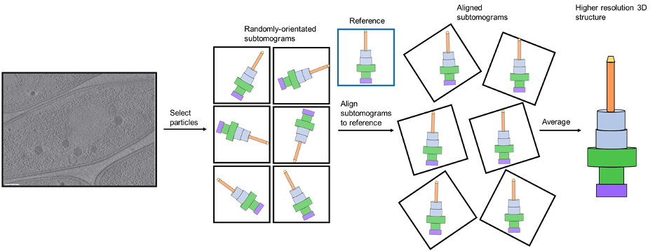
Figure 11: The workflow of subtomogram averaging. Protein particles are selected from a tomogram (example borrowed from a review by Melia and Bharat), resulting in the acquisition of randomly orientated subtomograms. These are aligned and averaged to produce the final 3D structure. Here, a simplistic model of a large multiprotein bacterial complex called a Type III secretion system is used as an example.
The major advantage of this technique is its ability to visualise protein structures in their native environment. In essence, the ‘big three’ techniques of structural biology – NMR, X-ray crystallography and single-particle analysis cryo-EM – are not capable of this since they require proteins to be extracted from cell expression systems and purified.
Proteins in solution are not always representative of their native cellular environment. This is because cells are extremely crowded and dynamic, so proteins may require particular cellular conditions or binding partners to adopt particular conformations and carry out particular functions. Hence, capturing protein structures in cells can lead to more functional insights compared to studying them in isolation. Furthermore, subtomogram averaging can be used to examine protein structures during cellular processes, such as mitosis or DNA repair.
While subtomogram averaging could provide unprecedented insight into protein structures, it is not yet capable of routinely obtaining structures with resolutions comparable to traditional single particle analysis.
There are many reasons for this. One reason is that the electrons from the beam are distributed across an entire tilt series, as opposed to an unmoving grid in single-particle analysis. Consequently, the electron dosage for each tomogram is lower, so the amount of useful information is lowered, worsening the resolution.
Another key problem is that subtomogram averaging is low throughput. What this means is that there may be very few images of particles that can be extracted from a tomogram. Single-particle analysis does not have this problem since large quantities of protein are recombinantly expressed. Having fewer particles means that the averaged subtomograms will have a lower signal-to-noise ratio and therefore, worse resolution.
Regardless, a lot of research is underway to improve the technology and image processing software for subtomogram averaging. In fact, improvements are beginning to bear fruit with numerous recent examples of structures at a comparable resolution to single-particle analysis. At this rate, routinely using subtomogram averaging to look at protein structures in their native cellular environments may soon be in reach.
MicroED
MicroED stands for microcrystal electron diffraction and is a form of electron crystallography. Electron crystallography is very similar to X-ray crystallography with one difference being that electrons are used instead of X-rays. Hence, the diffraction of electrons from crystals is recorded and used to work out the structure of proteins.
Historically, 2D crystals (crystals that consist of a layer that is one protein thick) were used with some success, the most famous of which is a 3.5 Å structure of bacteriorhodopsin – a bacterial light-sensing protein – by Henderson and his team in 1990.
Since then, 2D electron crystallography has been superseded by microED, whereby MicroED uses small 3D crystals instead. Normally, the signal from these small crystals would be too weak to be detected in X-ray crystallography; but because electrons interact more strongly with matter, a diffraction pattern can still be obtained to solve the structure.
A diagram of the process is shown below:
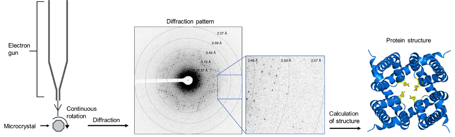
Figure 12: An overview of microED. Electrons are diffracted by a microcrystal undergoing continuous diffraction. From this, a diffraction pattern is produced which encodes the structural information of the protein. The positions of atoms can be calculated from this diffraction pattern, producing the structure of the protein. The example diffraction pattern and structure is a cation channel from an article by Liu and Gonen.
This technique has been used to solve structures with resolutions comparable to X-ray crystallography. For example, the structure of a cation channel from Liu and Gonen in 2018 was solved at a resolution of 2.5 Å. Furthermore, microED does not require large crystals like X-ray crystallography. For comparison, the diameters of crystals for X-ray crystallography are on the micrometre scale while the diameters of crystals for microED are on the nanometre scale. Forming large crystals is a major bottleneck in X-ray crystallography, so microED may be a useful alternative for obtaining structures from crystals that normally be considered ‘bad’ for X-ray crystallography.
However, coaxing proteins to form crystals (even very small ones) is still no easy feat.
MicroED also suffers the same phase problem as X-ray crystallography. This refers to how only the intensities (and hence, amplitudes) of electrons or X-rays scattered from a crystal can be recorded. In other words, the phase shifts are lost when collecting diffraction data, which is problematic since phase shifts are more important for working out the structure. Most structures solved by microED thus far have used molecular replacement – obtaining phases from a protein with a similar structure - to solve the phase problem. This means that solving the phase problem will be much more challenging for structurally characterising novel proteins. Furthermore, the enormous successes of single-particle analysis cryo-EM, cryo-ET and subtomogram averaging unfortunately means that microED has largely been overshadowed and is currently a relatively niche technique.
Henceforth, it remains to be seen whether it will stay this way or whether it will become a routinely-used technique in the future.
But really, this may just be the beginning of the cryo-EM story
Overall, cryo-EM is an evolving technique that encompasses biophysics, mathematics, computing and more.
But most importantly, cryo-EM is a powerful structural biology technique, which allows us to solve the structure of complex macromolecules at increasingly high resolution. Not only does this give us unprecedented insight into the molecular mechanisms of these biological molecules, but it also informs on drug discovery.
Similar principles to single-particle cryo-EM can be applied to cryo-ET and subtomogram averaging, enabling visualisation of larger cellular structures and macromolecules in their cellular environment. Furthermore, microED can be used as an alternative to X-ray crystallography to solve structures of proteins that are difficult to crystallise.
Here we have presented an overview of how cryo-EM works. However, do keep in mind each variant of cryo-EM, be it single particle analysis, cryo-ET or microED, is a field of active research. Much work has been done towards improving cryo-EM technology to achieve atomic resolution as well as using cryo-EM to answer biological problems.
With the ever-increasing number of cryo-EM structures in the Protein Data Bank (PDB) alongside the continuous advances in software, technology and methodologies, the future of cryo-EM looks bright.
Authors
Amy Cheng & Matthew Tang
BSc Biochemistry
Imperial College London


