
Green Fluorescent Protein: The BFF of Biochemistry
- Devyani Saini

- Jan 27, 2021
- 6 min read
Updated: Jul 6, 2023
In biochemistry research, proteins are frequently ‘tagged’ to track their location and discern other characteristics like cell morphology or function. There are various types of protein tags, one of which is a fluorescent tag. Fluorescent tags are useful as they give a simple colour output that can be viewed using a fluorescence microscope, as opposed to antibody tags which require primary and secondary antibody washes.
Green fluorescence protein (GFP), in particular, revolutionised molecular biology and cell biology research as a protein tag and reporter of gene expression, whereby it is frequently used in all branches of biochemical and biological research.
GFP was discovered accidentally (not unlike many great discoveries!) by Osamu Shimomura in 1962. Shimomura’s team was investigating a bioluminescent protein in the jellyfish Aequorea victoria termed aequorin. Upon purifying aequorin, the scientists also found an unknown protein that exhibited green fluorescence under UV light. This protein was later named GFP. In the jellyfish, the aequorin protein produced blue light, and this energy was transferred to the GFP, which emitted green light.
Further studies into GFP
Later, in 1979, Shimomura published an article on the structure of the GFP chromophore, which essentially showcases the specific molecular group(s) within the protein structure that causes GFP to be coloured.
Some fluorescent proteins only emit fluorescence in the presence of an external fluorophore cofactor (example: phycobiliproteins). External fluorophores are not a part of the protein itself, but a separate, non-protein molecule that interacts with the protein and allows it to fluoresce. GFP, however, contains the fluorophore within its amino acid chain and is thus able to spontaneously fluoresce upon folding of the protein into its native state.
However, despite this discovery, there was no significant research into GFP for 30 years after its discovery by Shimomura. Then, in 1992, Douglas Prasher cloned the GFP gene from A. victoria, paving the way for new research into this unique fluorescent protein. Cloning means essentially duplicating the DNA sequence of the GFP gene from the jellyfish’s DNA template so that the DNA of GFP can be investigated on its own.
The next milestone was reached by Martin Chalfie in 1994, who was able to clone GFP into Escherichia coli (a species of bacteria) and Caenorhabditis elegans (a species of roundworm) and see the fluorescence. He then concluded that GFP expression could be used to track protein location and analyse gene expression in vivo (i.e. in cells existing in their natural environment).
Cloning GFP into E. coli and C. elegans requires the use of a plasmid system. The plasmid (circular DNA) contains the gene of interest (GFP) and an antibiotic resistance cassette to select for positive clones, i.e. any cells which do not take up the plasmid will die in medium containing antibiotics because they will also not have taken up the antibiotic resistance gene!
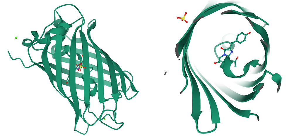
Figure 1: The structure of GFP. (Left) Side view of the ß-barrel structure of GFP. The green dot represents a calcium ion. (Right) Top view through the ß-barrel, revealing the chromophore (shown as sticks) in the centre. Yellow and red sticks (top left corner) represent a sulfate ion.
The functional mechanism of GFP
GFP is a 26.9 kDa protein with 238 amino acid residues and a distinct anti-parallel ß-barrel structure. The chromophore is formed after a post-translational modification (an attribute or physical trait of the protein that is added after it has been translated from mRNA by a ribosome) and is composed of the three amino acids Serine-65, Tyrosine-66, and Glycine-67. The secondary structure of the chromophore area is slightly helical, but not a complete alpha helix.
The proposed mechanism of fluorophore formation (see Figure 2) starts with a nucleophilic attack on the carbon atom of the S65 Carbonyl group (CO) by the G67 amide nitrogen. This creates an imidazolone ring. The S65 carbonyl oxygen is then lost in the form of a water molecule, and the Y66 is oxidized (i.e. loses electrons) by air to conjugate the system.
A conjugated system is a series of atoms in a molecule with connected p-orbitals (specifically sp2 orbitals), where the electrons are delocalized. They are often characterised by a series of carbon-carbon alternating double bonds. Conjugated systems can absorb different wavelengths of light depending on how conjugated it is (i.e. How many C=C bonds there are). The spontaneous formation of the conjugated ring in GFP is what allows it to absorb visible light and emit a visible colour.
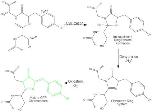
Figure 2: Mechanism of GFP fluorescence. The fluorophore is highlighted in green. [Source]
Improving wild-type GFP
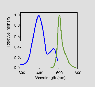
Figure 3: Excitation (blue) and emission (green) spectra of wild-type GFP. [Source]
Wild-type GFP from A. victoria absorbs light at 395 nm and emits at 509 nm. It has another small absorption peak at 475 nm, but the amplitude (and therefore intensity) is much lower than the peak at 395 nm.
It is known that absorption peaks of a longer wavelength are more photostable (i.e. resistant to change in the presence of light/radiation). Hence, in 1995, Robert Tsien’s group made a few point mutations (changing the amino acid at a specific position) in WT-GFP to make it more efficient and found that mutating the chromophore serine to threonine (S65T) resulted in a longer wavelength absorption peak (490 nm) and an amplitude six times greater than the wild-type protein. Longer wavelengths, as previously mentioned, are more photostable. Higher amplitude results in higher intensity, which would make the emission spectrum brighter, and thus easier to see through a fluorescence microscope.
However, the development of GFP didn’t stop there (in fact, that was only the beginning)!
In 1996, Zhang’s group added an additional mutation besides S65T - phenylalanine at position 64 was converted to leucine (F64L), which increased the protein folding efficiency. The resultant mutant was termed “EGFP (enhanced GFP)” and it exhibited fluorescence 35 times brighter than WT-GFP. EGFP absorbs light at 488 nm and emits at 509 nm. Many other studies tackled the same issue, and several enhanced versions of GFP were optimised for different applications.
But what if we want to track multiple proteins or understand the expression of multiple genes at the same time? Once again, GFP provides the solution.
Mutating GFP was also able to produce colour mutants, including blue (e.g. Azurite, BFP), yellow (e.g. Citrine, Venus), cyan (e.g. mTurquoise), and red (e.g. mCherry). Different colours are obtained by changing the amino acids in and around the protein’s chromophore (residues 63 to 66). This will change the band of the spectrum where GFP absorbs and emits light, thus changing its visible colour.
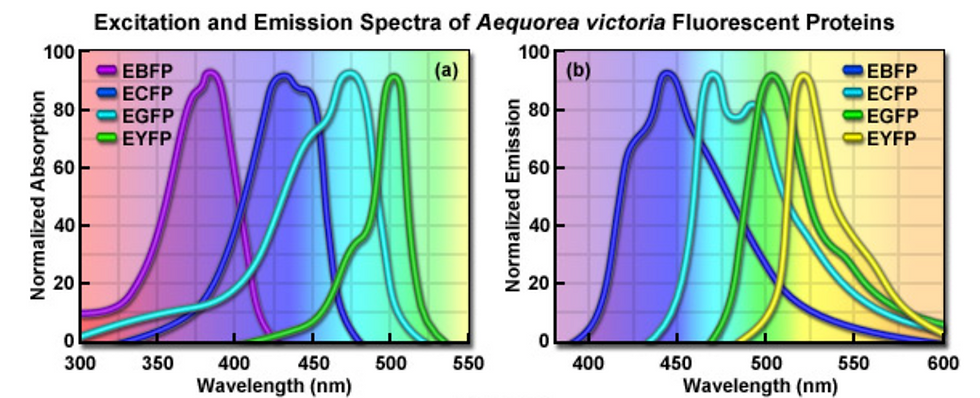
Figure 4: Excitation and emission spectra of enhanced GFP variants. [Source]
After adjusting and optimising each protein to obtain maximum brightness and efficiency, a substantial library of fluorescent proteins has been created for a myriad of molecular biology functions, and certain variants are still being developed today!
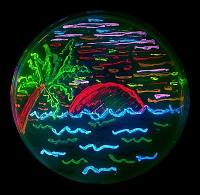
Figure 5: Beach scene drawn with bacteria expressing different colour mutants of GFP. [Source]
Visualising GFP experimentally
GFP and its variants are visualised using a fluorescence microscope. Fluorescence microscopes have a very bright light source such as a xenon lamp which can emit a large range of wavelengths from UV to infrared. The light source sends a beam towards an excitation filter, which will filter out all wavelengths besides the chosen excitation wavelength of the sample. Most modern fluorescence microscopes have built-in cameras to take images of the samples for data analysis and use in publications.
In the case of EGFP this would be set to 488 nm. The filtered beam of light will be directed to the sample via an angled mirror, and the sample will emit a resultant beam. This emitted beam will hit an emission filter above the sample, which will filter out all wavelengths besides the specific emission wavelength, in the case of EGFP this would be 509 nm. Due to the filtering, only the fluorescent parts of the image will be seen through the observation lens of the microscope!
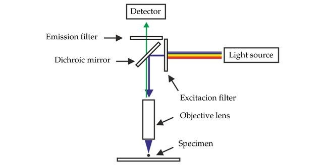
Figure 6: A schematic of the essential parts of a fluorescence microscope. [Source]
Besides that, GFP can also be visualised using flow cytometry. Flow cytometry is a cell-based analytical tool used to analyse a huge number of cells. Flow cytometry works by suspending cells in a fluid and running them past a laser beam one cell at a time. Each laser emits the excitation wavelength of the sample of interest, and the resultant fluorescence is captured by the instrument for analysis. The difference in using flow cytometry to analyse GFP fluorescence instead of microscopy is that flow cytometry can detect the amount of fluorescence in a quantitative way, whereas with microscopy the application is mainly for looking at the location of the target. Detecting the amount of fluorescence is useful in experiments where you want to understand increases and decreases in gene expression in response to variable factors, which will result in a corresponding change in fluorescence.
Concluding remarks
The beauty of GFP is that it can be easily fused to proteins at the N or C terminus and fluoresces spontaneously upon folding. These properties make it a useful tool to track proteins in their native environments. It can also be added downstream of a gene promoter to look at transcriptional activation (i.e., when there is transcription, there will be fluorescence).
The discovery and development of GFP as a research tool is marked as a significant milestone in the history of biochemical research, and was awarded the 2008 Nobel Prize in Chemistry jointly to Osamu Shimomura, Martin Chalfie, and Roger Tsein. Nonetheless, this brief introduction has only highlighted a fraction of the applications and significance of this interesting and useful protein, which is often taken for granted in the research space.
Author
Devyani Saini
MRes Molecular & Cellular Biosciences
Imperial College London


